Difference between revisions of "MATLAB:Logical Masks"
| Line 232: | Line 232: | ||
f: [ 0 0 0 1 2 3 4 5 5 5 5 5 5 7 9] | f: [ 0 0 0 1 2 3 4 5 5 5 5 5 5 7 9] | ||
</source> | </source> | ||
| + | ==== Simplification ==== | ||
| + | Once again, the code above takes up far more space than it needs to in order to individually calculate each component part of the solution. In practice, the code would be: | ||
| + | <source lang="matlab"> | ||
| + | x = -2:12 | ||
| + | f = ... | ||
| + | (x<0) .* (0) + ... | ||
| + | (0<=x & x<5) .* (x) + ... | ||
| + | (5<=x & x<10) .* (5) + ... | ||
| + | (x>=10) .* (2*x-15); | ||
| + | stem(x, f) | ||
| + | axis([-3 13 -1 10]) | ||
| + | xlabel('x') | ||
| + | ylabel('f(x)') | ||
| + | title('f(x) (NET ID)') | ||
| + | print -deps PFunction | ||
| + | </source> | ||
| + | |||
===Example 2 - Acceleration Due To Gravity === | ===Example 2 - Acceleration Due To Gravity === | ||
Revision as of 17:38, 10 September 2013
Contents
Introduction
Many times, you will see functions that are written in some kind of piecewise fashion. That is, depending upon that value of the input argument, the output argument may be calculated in one of several different ways. In these cases, you can use MATLAB's logical and relational arguments to create logical masks - matrices containing either 0's or 1's - to help determine the appropriate calculation to perform to determine the values in a matrix.
Important Note
The examples in Piecewise Constant and Non-constant Piecewise Functions use scripts and are not creating functions. To see how to create a function that employs logical masks, pay particular attention to Using Logical Masks in Functions and especially note that all the mask and function calculations are performed inside the function.
Piecewise Constant
Sometimes, piecewise functions are broken up into several regions, with each region being defined by a single constant. These are called piecewise constant functions and can be easily generated in MATLAB.
Example - GPA Calculation
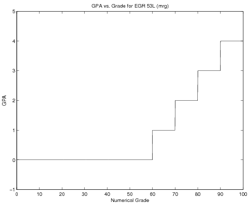
Take for example GPA as a function of numerical grade (assume \(\pm\)do not exist for the moment...). The mathematical statement of GPA might be:
\( \mbox{GPA}(\mbox{Grade})=\left\{ \begin{array}{rl} \mbox{Grade}\geq 90~~~ & 4.0\\ 80\leq\mbox{Grade} ~\And~ \mbox{Grade}<90~~~ & 3.0\\ 70\leq\mbox{Grade} ~\And~ \mbox{Grade}<80~~~ & 2.0\\ 60\leq\mbox{Grade} ~\And~ \mbox{Grade}<70~~~ & 1.0\\ \mbox{Grade}<60~~~ & 0.0 \end{array} \right. \)
If you want to write this table as a function that can accept multiple
inputs at once, you really should not use an if-tree
(because if-trees can only run one program segment for the entire matrix) or a
for loop (because for loops are slower and more complex
for this particular situation).
Instead, use MATLAB's ability to create logical masks. Look
at the following code:
Grade=linspace(0, 100, 1000);
MaskForA = Grade>=90;
The variable MaskForA will be the same size of the Grade
variable, and will contain only 0's and 1's -- 0 when the logical
expression is false and 1 when it is true. Given that, you can use
this in conjunction with the function for an "A" grade to start
building the GPA variable:
Grade=linspace(0, 100, 1000);
MaskForA = Grade>=90;
FunctionForA = 4.0;
GPA = MaskForA.*FunctionForA;
At the end of this code, the GPA variable will contain a 4.0
wherever the logical mask MaskForA was a 1 and it will contain a
0.0 wherever the logical mask was a 0. All that is required is to
extend this to the rest of the possible GPA's - the full code is in the section below, along with an image of the graph it will create. Note the use of the continuation ... to write the commands in the same
visual way the function definition is written - this is not required, but
does make the code easier to interpret.
Also, the axes of the graph have been changed using the axis
command so that the graph is not directly on top of the border of the
plot. Without this change, the "A" portion of the graph would be
hidden by the top edge of the figure boundary.
Code and Graph
Grade=linspace(0, 100, 1000);
MaskForA = Grade>=90;
FunctionForA = 4.0;
MaskForB = 80<=Grade & Grade<90;
FunctionForB = 3.0;
MaskForC = 70<=Grade & Grade<80;
FunctionForC = 2.0;
MaskForD = 60<=Grade & Grade<70;
FunctionForD = 1.0;
MaskForF = Grade<60;
FunctionForF = 0.0;
GPA = ...
     MaskForA.*FunctionForA + ...
     MaskForB.*FunctionForB + ...
     MaskForC.*FunctionForC + ...
     MaskForD.*FunctionForD + ...
     MaskForF.*FunctionForF;
plot(Grade, GPA)
axis([0 100 -1 5])
xlabel('Numerical Grade')
ylabel('GPA')
title('GPA vs. Grade for EGR 103L (mrg)')
print -deps GPAPlot
For a further explanation, look at the following code (which involves fewer points which are not in any particular order):
ClassGrades=[95 70 68 38 94 84 92 87];
MaskForA = ClassGrades>=90;
FunctionForA = 4.0;
MaskForB = 80<=ClassGrades & ClassGrades<90;
FunctionForB = 3.0;
MaskForC = 70<=ClassGrades & ClassGrades<80;
FunctionForC = 2.0;
MaskForD = 60<=ClassGrades & ClassGrades<70;
FunctionForD = 1.0;
MaskForF = ClassGrades<60;
FunctionForF = 0.0;
GPA = ...
     MaskForA.*FunctionForA + ...
     MaskForB.*FunctionForB + ...
     MaskForC.*FunctionForC + ...
     MaskForD.*FunctionForD + ...
     MaskForF.*FunctionForF;
The masks now looks like:
MaskForA: [1  0  0  0  1  0  1  0]
MaskForB: [0  0  0  0  0  1  0  1]
MaskForC: [0  1  0  0  0  0  0  0]
MaskForD: [0  0  1  0  0  0  0  0]
MaskForF: [0  0  0  1  0  0  0  0]
and the product of each of the masks with each of the functions produces:
MaskForA.*FunctionForA: [4  0  0  0  4  0  4  0]
MaskForB.*FunctionForB: [0  0  0  0  0  3  0  3]
MaskForC.*FunctionForC: [0  2  0  0  0  0  0  0]
MaskForD.*FunctionForD: [0  0  1  0  0  0  0  0]
MaskForF.*FunctionForF: [0  0  0  0  0  0  0  0]
These five matrices are added together to give:
GPA: [4 2 1 0 4 3 4 3]
Simplification
You do not need to give each mask and function a name - rather, you can compute the masks and multiply them by their appropriate function segments, all in one function line. For example, the GPA variable above could be calculated as:
Grade=linspace(0, 100, 1000);
GPA = ...
     (Grade>=90)            .* (4.0) + ...
     (80<=Grade & Grade<90) .* (3.0) + ...
     (70<=Grade & Grade<80) .* (2.0) + ...
     (60<=Grade & Grade<70) .* (1.0) + ...
     (Grade<60)             .* (0.0)
Just make sure each mask is surrounded by parenthesis, each function segment (in this case, a constant) is surrounded by parenthesis, and the appropriate masks and function segments are element multiplied.
Non-constant Piecewise Functions
Sometimes, piecewise functions are defined as following different formulas involving the independent variable over a range of inputs rather than being piece-wise constant.
Example 1 - Discrete Function
For example, the expression:
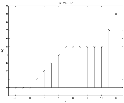
\( f(x)=\left\{ \begin{array}{rl} x<0 & 0\\ 0\leq x<5 & x\\ 5\leq x<10 & 5\\ x\geq 10 & 2x-15 \end{array} \right. \)
which, for integers -2:1:12 can be calculated and graphed:
Code and Graph
x = -2:12
Mask1 = x<0;
Function1 = 0;
Mask2 = (0<=x) & (x<5);
Function2 = x;
Mask3 = (5<=x) & (x<10);
Function3 = 5
Mask4 = x>=10;
Function4 = 2*x-15;
f = ...
     Mask1.*Function1 + ...
     Mask2.*Function2 + ...
     Mask3.*Function3 + ...
     Mask4.*Function4;
stem(x, f)
axis([-3 13 -1 10])
xlabel('x')
ylabel('f(x)')
title('f(x) (NET ID)')
print -deps PFunction
Several of these variables are presented below. Note that the spacing
in this document is set to make it easier to see which elements in one variable are
paired up with equivalent elements in another variable (for example,
to determine the element-multiplication of Mask2 and Function2).
Given the code above, the masks are:
Mask1: [  1   1   0   0   0   0   0   0   0   0   0   0   0   0   0]
Mask2: [  0   0   1   1   1   1   1   0   0   0   0   0   0   0   0]
Mask3: [  0   0   0   0   0   0   0   1   1   1   1   1   0   0   0]
Mask4: [  0   0   0   0   0   0   0   0   0   0   0   0   1   1   1]
Notice how the masks end up spanning the entire domain of \(x\) without overlapping. The functions - as calculated over the entire domain, are:
Function1: [0]
Function2: [ -2  -1   0   1   2   3   4   5   6   7   8   9  10  11  12]
Function3: [5]
Function4: [-19 -17 -15 -13 -11  -9  -7  -5  -3  -1   1   3   5   7   9]
The individual products of the masks and the functions give:
Mask1.*Function1: [  0   0   0   0   0   0   0   0   0   0   0   0   0   0   0]
Mask2.*Function2: [  0   0   0   1   2   3   4   0   0   0   0   0   0   0   0]
Mask3.*Function3: [  0   0   0   0   0   0   0   5   5   5   5   5   0   0   0]
Mask4.*Function4: [  0   0   0   0   0   0   0   0   0   0   0   0   5   7   9]
Finally, when these are all added together, none of the individual products interfere with each other, so:
f: [ 0 0 0 1 2 3 4 5 5 5 5 5 5 7 9]
Simplification
Once again, the code above takes up far more space than it needs to in order to individually calculate each component part of the solution. In practice, the code would be:
x = -2:12
f = ...
   (x<0)         .* (0) + ...
   (0<=x & x<5)  .* (x) + ...
   (5<=x & x<10) .* (5) + ...
   (x>=10)       .* (2*x-15);
stem(x, f)
axis([-3 13 -1 10])
xlabel('x')
ylabel('f(x)')
title('f(x) (NET ID)')
print -deps PFunction
Example 2 - Acceleration Due To Gravity
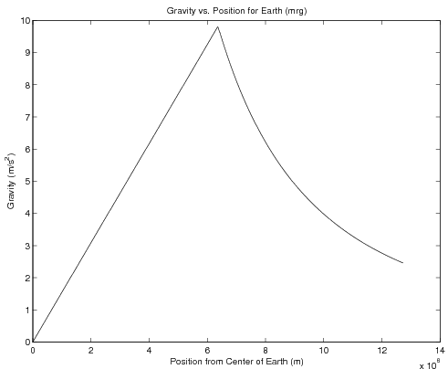
The following example determines the acceleration due to gravity for a sphere a particular distance away from the center of a sphere of constant density \(\rho\) and radius R. The formula changes depending on whether you are inside the sphere's surface or not. That is:
\( \mbox{Gravity}(r)= \left\{ \begin{array}{lr} r<=R & \frac{4}{3}\pi G\rho r\\ r>R & \frac{4}{3}\pi G \rho\frac{R^3}{r^2} \end{array} \right. \)
You can use the same method as the example above, making sure to calculate the values of the function rather than simply using constants. The following code and graph demonstrate:
Code and Graph
G = 6.67e-11; rho = 5515; R = 6371e3;
Position=linspace(0, 2*R, 1000);
MaskForInside = Position<=R;
FunctionForInside = 4/3*pi*G*rho*Position;
MaskForOutside = Position>R;
FunctionForOutside = 4/3*pi*G*rho*R.^3./Position.^2;
Gravity = ...
     MaskForInside.*FunctionForInside + ...
     MaskForOutside.*FunctionForOutside;
plot(Position, Gravity, 'k-');
xlabel('Position from Center of Earth (m)');
ylabel('Gravity (m/s^2)');
title('Gravity vs. Position for Earth (mrg)');
print -deps GravityPlot
Note that this code will generate a warning since the first value of
Position is 0 and the second function requires division by that
variable. Still, this is just a warning, and MATLAB does produce the
plot shown above, despite the warning.
Using Logical Masks in Functions
Any of these tasks can be done using inline functions or function files. For the gravity example,
you could create a function - say, GravFun.m for this problem. Regarding simplifying the code, as mentioned above, make sure each mask is surrounded by parentheses, each function segment is surrounded by parentheses, and the appropriate masks and function segments are element multiplied.
In that case, your function file and script file might be:
|
Function file, GravFun.m function out = GravFun(r, rho, R)
G = 6.67e-11;
out = (r<=R) .* (4/3*pi*G*rho*r) + ...
(r>R) .* (4/3*pi*G*rho*R.^3./r.^2);
|
Script file, RunGravFun.m rho = 5515; R = 6371e3;
Position=linspace(0, 2*R, 1000);
Gravity = GravFun(Position, rho, R);
plot(Position, Gravity, 'k-');
xlabel('Position from Center of Earth (m)');
ylabel('Gravity (m/s^2)');
title('Gravity vs. Position for Earth (mrg)');
print -deps GravityPlot2
|
You could also write an anonymous function in a script to compute the gravity:
rho = 5515; R = 6371e3; G = 6.67e-11;
Position=linspace(0, 2*R, 1000);
GravFun = @(r, rho, R) (r<=R) .* (4/3*pi*G*rho*r) + ...
                 (r>R)  .* (4/3*pi*G*rho*R.^3./r.^2);
Gravity = GravFun(Position, rho, R);
plot(Position, Gravity, 'k-');
xlabel('Position from Center of Earth (m)');
ylabel('Gravity (m/s^2)');
title('Gravity vs. Position for Earth (mrg)');
print -deps GravityPlot3
Note in this case the constants rho, R, and G need to
be defined before the anonymous function is created.
Questions
Post your questions by editing the discussion page of this article. Edit the page, then scroll to the bottom and add a question by putting in the characters *{{Q}}, followed by your question and finally your signature (with four tildes, i.e. ~~~~). Using the {{Q}} will automatically put the page in the category of pages with questions - other editors hoping to help out can then go to that category page to see where the questions are. See the page for Template:Q for details and examples.


